-
Notifications
You must be signed in to change notification settings - Fork 28
Advanced events and pre equilibration
This chapter will serve as a basic introduction to the event system added in revision 3/26/2015. You can find the code for this introduction in /examples/Advanced_Events.
The D2D framework allows incorporation of so-called events. Typically, events are characterized by a sudden change in a concentration, state or input. Depending on how the system is modeled, such events can induce sudden (near) discontinuities in the model simulations. Considering that the ODE solver uses automatic step size control, this can be problematic as the simulation may skip over aforementioned events. Rather than limiting the step size manually, it is better to specify such events. This signals the solver to only integrate up to the point of the event and then re-initialize the integrator to perform the remainder of the simulation.
This short tutorial will provide an introduction to incorporating dynamic events in the model. Using the event system requires some familiarity with the D2D framework. However, it is well suited for dynamic changes to the model since adding or removing events does not require the model to be recompiled. Events provide direct access to the model states at any point in time and invoke re-initialization of the ODE solver. As such, they are a powerful mechanism to introduce abrupt changes in the system. Certain aspects of the event system have been automated. For example, to automatically scan the model inputs for step functions and mark these as events, invoke the command arFindInputs.
This tutorial will go into more advanced applications of the event system. To run the examples in this tutorial, we first initialize the D2D framework, load a model and compile it. We also set a few parameters.
arInit;
arLoadModel('events');
arCompileAll;

arSetPars('k_prod', .2);
arSetPars('k_deg', -3);
arSetPars('k_tr', -0.5);
Events can be added using the arAddEvent command. This command adds an event to a condition. An event is added for a specific condition at a specific time point. In this example, we only have one model and one condition; hence the first two arguments are both 1. The third argument refers to the time point at which the event is supposed to occur. We could stop here; which would add the event (a point where the solver is re-initialized), but not changing any of the state variables. This can be useful for making sure that simulations remain accurate around abrupt input changes (such as step functions).
However, in this example, we would like to perturb the system at these events. To do this, we can use the last three arguments, which correspond to the name of the state we wish to change (in this case stateA or stateB) and the coefficients corresponding to a linear equation of the form aX+b; where X represents the old state variable. Note that instead of a state identifier, we could have also supplied a numeric vector, which corresponds to state indices.
arAddEvent(1, 1, 50,  'stateA', 1,  10);    % Add 10A at t=50 [A=(1*A+10)]
arAddEvent(1, 1, 60,  'stateA', 0.5 );      % Double the volume (half the concentration) at t=60 (A=(0.5*A))
arAddEvent(1, 1, 60,  'stateB', 0.5 );      % Doubling the volume also has to be taken into account for state B (B=(0.5*B))
arAddEvent(1, 1, 70,  'stateA', 1,  10);    % Add some A at t=70
arAddEvent(1, 1, 80,  'stateA', 0.5 );      % Double the volume (half the concentration) at t=80
arAddEvent(1, 1, 80,  'stateB', 0.5 );
arAddEvent(1, 1, 90,  'stateA', 1,  10);    % Add some A at t=90
arAddEvent(1, 1, 100, 'stateA', 0.5 );      % Double the volume (half the concentration) at t=100
arAddEvent(1, 1, 100, 'stateB', 0.5 );
arAddEvent(1, 1, 110, 'stateA', 1,  10);    % Add some A at t=110
arAddEvent(1, 1, 120, 'stateA', 0.5 );      % Double the volume (half the concentration) at t=110
arAddEvent(1, 1, 120, 'stateB', 0.5 );
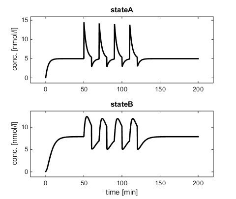
If we now simulate the system, we can see the effect of our events:

See d2d\arFramework3\Examples\ToyModels\Input_Tests\Models\input_tests.def:
INPUTS
BolusInjection   C  nM  conc.  "bolus(t, bolus_amount, injection_timepoint, injection_duration)"
Step             C  nM  conc.  "step1(t, pre_step, 50, post_step)"
TwoStep          C  nM  conc.  "step2(t, pre_step, 25, pre_step+step_size, 50, pre_step+2*step_size )"
SmoothStep       C  nM  conc.  "smoothstep1(t, pre_step, 50, post_step, smoothness)"
SmoothTwoStep    C  nM  conc.  "smoothstep2(t, pre_step, 25, pre_step+step_size, 50, pre_step+2*step_size, smoothness)"
Smooth1          C  nM  conc.  "smooth1(t, 40, 50)"
Smooth2          C  nM  conc.  "smooth2(t, 40, 50)"
ThreeStep        C  nM  conc.  "step3(t, pre_step, 25, pre_step+step_size, 50, pre_step+2*step_size,75,pre_step+3*step_size )"
FourStep         C  nM  conc.  "step4(t, pre_step, 15, pre_step+step_size, 30, pre_step+2*step_size,45,pre_step+3*step_size,60,pre_step+4*step_size )"
PeriodicStep     C  nM  conc.  "periodicstep(t,90,10,5)"
In D2D, a condition is defined as a model in combination with a specific set of parameter transformations and initial condition. One condition typically results in one simulation. Quite often, one data set gives rise to several conditions (e.g. dose response data). Conversely however, conditions may be shared among multiple data sets. This saves simulation time when many datasets make use of the same conditions. However, if one wishes to set an event for one specific dataset and not the other; but the two share conditions, then this is a problem. When this happens, it is important to invoke arSplitDataConditions with the appropriate parameters, before assigning events. arSplitDataConditions splits the conditions corresponding to a list of data indices; such that these datasets get their own unique conditions. These data indices can be found by issuing the command arFindData with a string that (partially) matches the dataset's filename.
arSplitDataConditions( model, dataIDs, verbose )
Note that arSplitConditions cannot be undone without recompilation of the model.
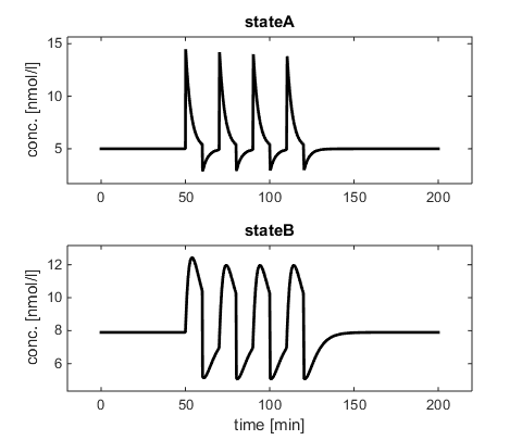
One thing we notice is that the system is not in steady state prior to the events. Let's, for demonstration purposes, assume that we wish to ensure that the system is in steady state prior to the event. One approach would be to algebraically encode the steady state in the model definition files by means of parameter transformations. When possible, this is the preferred approach, since it automatically takes into the account the steady state without any simulation requirements. However, in some practical cases, the steady state equations may be too complex to determine beforehand. In such cases, pre-simulation provides an answer. Again; there are two ways of dealing with this. If the system equilibrates quickly, and all feasible parameter values correspond to short equilibration times, one can simply start the simulation at negative time. This would give the system some time to equilibrate before the first input is applied. However, when the parameters are largely unknown, this is often not an option, since the equilibration time might depend strongly on the parameters we wish to infer. In such cases, the event-based equilibration system provides a solution.
Event based pre-equilibration corresponds to simulating the system (and also the sensitivity equations) up to steady state prior to simulating the true system. Pre-equilibration uses separate conditions for this (stored in a subfield ss_condition). These conditions are based on copies of conditions that are already present in the model. After the equilibration has been performed for all steady state conditions, the final values for the states and sensitivities are copied as initial values for the relevant target conditions (using the event system). Long story short, the command to invoke pre-equilibration steps is arSteadyState.
Let's add a pre-equilibration step:
arSteadyState(1,1,1);
Here we add a steady state pre-equilibration for model 1 (first argument), where we use condition 1 as the source condition (second argument) and condition 1 as the target condition. If we now rerun the simulation, we observe that the system does start in steady state:

One important thing to note is that all the properties of a condition are copied. If a condition has an input, the steady state condition will also use that input. It is therefore practical to use a condition without input as source condition. Also note that the event system does not work during equilibration. Therefore, event based steps will be ignored for the equilibration condition.
How do I find which condition number to use as source and target?
The second example involves a slightly more realistic use case. Here, there are multiple data-sets and multiple conditions. First load the model and data:
arInit;
arLoadModel('equilibration');
arLoadData('cond1', 1, 'csv');
arLoadData('cond2a', 1, 'csv');
arLoadData('cond2b', 1, 'csv');

% Merge plots
arMergePlotMulti(1, {'cond1', 'cond2a', 'cond2b'}, ...
                    {'condition 1', 'condition 2', 'condition 2'}, ...
                    'plot' );

arCompileAll;

arSetPars('k_basal', 0);
arSetPars('k_deg', -1);
In order to find the appropriate condition for adding the event, we can invoke the command arShowDataConditionStructure. This provides us with the following output:
	data #1: cond1 -> condition #1
	amount = 1		input_bas_inh = 0

	data #2: cond2a -> condition #2
	amount = 1		input_bas_inh = 1

	data #3: cond2b -> condition #3
	input_bas_inh = 1
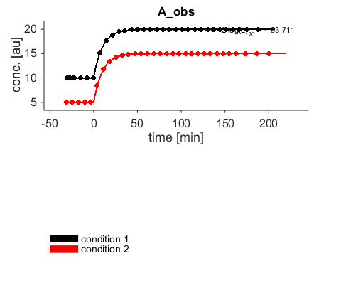
Here, condition 2 and 3 have a non-zero value for input_bas_inh, which represents an inhibition of basal activation and therefore correspond to a different steady state than condition 1. Also note that the model contains a step function; which requires us to invoke arFindInputs, to make sure that we reset the solver on the step function location.
arFindInputs;
We can now add the steady states:
arSteadyState(1, 1, 1, [], -1e7);
arSteadyState(1, 2, [2,3], [], -1e7);
Again, the first argument corresponds to the model, the second argument to the source condition and the third to the target condition. The fifth argument is optional and represents a starting time for the equilibration. In this case, we have a step function at t=0, and we want to make sure that the equilibration never reaches this step function. Hence, we start equilibration at -1e7. For this example, this is sufficient. For more complex models, a safer and preferable option would be to include conditions without input (e.g. with a stimulus dose of zero) and specifically use those for the equilibration step. Rather than hardcoding the condition numbers as demonstrated above, one can reference the relevant conditions by name using the function arFindCondition.
Example:
arSteadyState(1, arFindCondition(ar,'steady'), 'all');
Or even:
arSteadyState(1, arFindCondition(ar,'steady', 'input_A', 0, 'input_B', 5), 'all');
To select a specific condition when the reference dataset contains multiple conditions. Please see the help for arFindCondition for more optional flags and options. If we now simulate and plot the model (using arPlot), we see that the appropriate steady states have been taken into account.

By default, all values of a steady state equilibration are copied into the destination initial condition. In some cases, this is undesirable. If you wish to omit states; supply a cell array of state names that are to be omitted from the equilibration. Note however, that this can lead to the system initially not being in equilibrium in the target condition.
** Important note on number of initial condition parameters **
If you have conserved moieties in your system, that is, conserved pools of species whose total does not vary; only one initial condition parameter for each closed pool suffices. This initial will represent the total of the conserved moieties. For unconserved species, all initials can be set to zero as they will be equilibrated to their respective values. This results in a reduction of the number of parameters in the system.
I made a mistake/Added an event I didn't want/how do I get my old model back?
Simply invoke arClearEvents. This should remove all events and equilibration steps. If you completely want to shut the event system down, because you think you may be encountering a bug or some other problem, set ar.config.useEvents to 0. Please don't forget to report the bug to us too.
Tolerances
Finally, a word on tolerances. Equilibration is based on simulating the system until the right hand side of the differential equations falls below an absolute tolerance. This absolute tolerance can be set in ar.config.eq_tol and is set to 10^-8 by default. Equilibration will start by simulating 100 time units (ar.config.init_eq_step) and increasing this time by a factor of five every time the equilibration tolerance was not reached (ar.config.eq_step_factor). 20 of such increases of the equilibration time are attempted (ar.config.max_eq_steps). If the requested tolerance is achieved, the simulation proceeds as expected. If the tolerances cannot be met before reaching max_eq_steps, the simulation aborts and presents a simulation failure. If this happens, check whether a stable steady state actually exists. Finally, if for any reason, the duration of the equilibration step is required, it can be found in the ss_condition substructure; namely in the field tEq (Example: ar.model(1).ss_condition(1).tEq). The right hand side of the ODEs at the final equilibration attempt can be found in the subfield dxdt.
Faster equilibration
Various methods were implemented to speed up the process of pre-equilibration. The first is fast equilibration using the implicit function theorem. Here the sensitivity condition is simulated to steady state, without integrating the sensitivity equations. Then, at the final time point, the steady state sensitivities are computed via the implicit function theorem (in the function fastSteadyState in arSimu.m). This process requires solving a system of equations. For this to work reliably, dfxdx has to be full rank. Hence, if one wishes to use this method, it is highly recommended to specify the model in such a way that it does not contain conserved pools. This can be achieved by calling arReduce after arLoadModel. For large systems, simulating in this way can be orders of magnitude faster than simulating the complete system. To use this system set ar.config.turboSSSensi to 1. The second option is to use rootfinding, but this method is not that reliable when little is known about the system. If dfxdx is ill-conditioned or the system contains multiple steady states, this will typically not be reliable. To enable rootfinding, set ar.config.rootfinding to 1. There is also a C implementation of this which can be activated by setting ar.config.C_rootfinding to 1.
How are simulated steady states handled internally in D2D?
Simulated steady states were a feature which was introduced in later versions of D2D. For legacy reasons, the steady state simulation system was implemented in a way which may not be immediately obvious, hence the way the system works is detailed here.
Steady state pre-equilibrations are implemented as new conditions in ar.model(m).ss_condition(ssc). These conditions have a field named src, which tells the C code which condition has to be simulated for this steady state (it refers to a condition ID in ar.model.condition). The fine simulation points (stored in tFine) for these conditions are set to [tstart, inf]. This infinity signals the ODE solver to simulate the system to steady state at this point (the tolerances for this can be found in ar.config.eq_tol). In principle it can also be used in normal conditions, but this is a deliberately undocumented function since there is currently no integration test covering this behavior.
When arSimu (the main simulation function) is called, the ss_conditions are always simulated first. Then in a second step, the event system is used to transfer the final simulated values in xFineSimu and sxFineSimu for the sensitivities and state variables to the desired target conditions. This is implemented by assigning an event to the target conditions which overwrites the states and sensitivities at the initial condition. These overwrite commands are stored in the field modx_A, modx_B, modsx_A. modsx_B which correspond to setting the states and sensitivities to A * oldValue + B. Hence, in this case, A is set to 0 for this time point and B is set to the value it needs to be set to.
If for any reason you would like to add functionality or debug something, the state and sensitivity changes are stored in ar.model.condition.modx_A, modx_B, modsx_A and modsx_B. The time points for the event system are included in tFine and tExp upon linking with arLink. arAddEvent (which is called by arSteadyState) invokes model linking.
- Installation and system requirements
- Setting up models
- First steps
- Advanced events and pre-equilibration
- Computation of integration-based prediction bands
- How is the architecture of the code and the most important commands?
- What are the most important fields of the global variable ar?
- What are the most important functions?
- Optimization algorithms available in the d2d-framework
- Objective function, likelhood and chi-square in the d2d framework
- How to set up priors?
- How to set up steady state constraints?
- How do I restart the solver upon a step input?
- How to deal with integrator tolerances?
- How to implement a bolus injection?
- How to implement washing and an injection?
- How to implement a moment ODE model?
- How to run PLE calculations on a Cluster?