-
Notifications
You must be signed in to change notification settings - Fork 28
Raia_CancerResearch2011
Reference: Raia et al. Dynamic Mathematical Modeling of IL13-induced Signaling in Hodgkin and Primary Mediastinal B-cell Lymphoma Allows Prediction of Therapeutic Targets. Cancer Research 71, pp. 693-704, 2011.
Folder: /Examples/Raia_CancerResearch2011.
Facts: The model contains 205 data points, 39 free parameters and 4 experimental conditions.
This page provides a guided tour through the Data2Dynamics software using the dynamical model of JAK2/STAT5 signal transduction published in Raia et al., Cancer Research 2011.
Like most projects in Data2Dynamics this example is based on
- a model definition file specifying inputs, reactions, observations, and error model
- data definition files depicting experimental setups different from those defined previously
- data files containing the measured data
- a setup file to initialize the software, load model as well as data and create the associated C files
These definition, data and setup files are located in /Examples/Raia_CancerResearch2011,
and their respective subfolders.
The Data2Dynamics software works hierarchical in the sense that specifications in the model definition are considered as defaults but may be overwritten for particular data sets by specifications in the respective data definition file. If on the other hand a data definition file is empty except the mandatory keywords in capitals, the defaults from the model definition are used. The latter case is the situation in this example.
The following tasks are routinely performed after model and data have been loaded:
- Plotting to visualize the data and/or the dynamics generated from the current set of parameters
- Fitting to adjust the parameters to describe the data as good as possible
- Uncertainty analysis to assess parameter identifiability and calculate confidence intervals
The file il13_jak2_stat5.def in the /models subfolder specifies the ODE model, i.e.
names and units of the dynamic variables and their dynamic interactions by providing
reaction schemes. A model definition file is divided in several sections that are described
in detail at the Setting up models page. Most prominently the differential equation system is
defined in the REACTIONS section as conversion scheme.
...
REACTIONS
Rec             ->  IL13_Rec        CUSTOM "il13_level * Kon_IL13Rec * 2.265 * Rec"
Rec             ->  Rec_i           CUSTOM "Rec_intern * Rec"
Rec_i           ->  Rec             CUSTOM "Rec_recycle * Rec_i"
...
Each line represents a biochemical reaction. Reactants and products are specified on the
left and right of the reaction arrow -> and the reaction rate is specified next. Here, the
membrane associated receptor Rec either forms a complex IL13_Rec with the ligand
IL13 (first line) or is internalized (second line). The internalized receptor Rec_i is again
recruited to the membrane (third line). Each reaction rate is added to the right-hand-side of
the ODEs for the products and subtracted for the reactants. The Data2Dynamics software
parses the specified reaction rates and considers each term that is neither a dynamic variable
nor an input as parameter, which can be estimated later from the data. As il13_level is
set to the input dose for each experiment the introduced parameters from the reactions
above are Kon_IL13Rec, Rec_intern and Rec_recycle.
Later in the same file il13_jak2_stat5.def the observation functions are specified to make
the default connection between dynamic variables and experimental data. In particular the
observation functions are defined in the OBSERVABLES section and the associated error
model after the keyword ERRORS.
...
OBSERVABLES
RecSurf_obs			C   au  conc.   0   0   "Rec + IL13_Rec + p_IL13_Rec"
IL13_cell_obs		C   au  conc.   0   0   "scale_IL13_cell_obs * IL13_cell"
...
ERRORS
RecSurf_obs			"RecSurf_obs1 + RecSurf_obs2*RecSurf_obs"
IL13_cell_obs		"IL13_cell_obs1 + IL13_cell_obs2*IL13_cell_obs"
...
For example, the total amount of receptor on the surface is defined as the
observable RecSurf_obs. As the IL13 concentration can only be observed on a relative
scale, the observational parameter scale_IL13_cell_obs is introduced. For each
observable it is required to specify an error model, in this case a relative error
RecSurf_obs2*RecSurf_obs with an offset RecSurf_obs1 is implemented.
The file MedB1_real_data.def in the /data subfolder is empty except for keywords
hence the observables defined in the model definition above are not altered.
The associated file MedB1_real_data.xls contains the experimental data.
time	il13_level	pIL4Ra_obs	pJAK2_obs	IL13_cell_obs	RecSurf_obs		...
0.0		0			NaN			NaN			0.616			1.289752779
5.0		0			NaN			NaN			NaN				NaN
10.0	0			NaN			NaN			NaN				1.57854438
...
Note that the headers of this file must match either the independent variable (here: time),
or a model parameter (e.g. il13_level), or the name of an observable (e.g. RecSurf_obs).
Columns with unrecognized headers are ignored.
Executing the script Setup.m loads model and data in MATLAB and automatically
generates the C-files.
After the setup script is finished once, the full functionality of the Data2Dynamics
framework can be applied for the analyses. All information about model and data are now
available in the MATLAB environment as a global variable ar. Below some basic
functions are explained briefly, for further information see
[Extended Functionalities](Extended Functionalities) and
[Function Reference](Function Reference).
Calling arPrint shows the list of all model parameters in the MATLAB command window.
The output contains: the parameter index (#), a classifier (D=parameter involved in
dynamics, E=error model parameter), the parameter name, its current values (values),
upper bound (ub) and lower bound (lb), if the values are given on a log10-scale and the
respective non-log10 parameter value (10^value), if the parameter is free for fitting (fitted,
0=fix, 1=fitted, 2=constant), and the prior distribution for this parameter (prior).
Parameters: # = free, C = constant, D = dynamic, I = initial value, E = error model

           name                       lb       value       ub          10^value        fitted   prior
#   1|D  | CD274mRNA_production     |       -5       -1.7         +3 | 1     +0.021 |       1 | uniform(-5,3)
#   2|D  | DecoyR_binding           |       -5       -2.4         +3 | 1    +0.0039 |       1 | uniform(-5,3)
#   3|D  | JAK2_p_inhibition        |       -5       -1.1         +3 | 1     +0.078 |       1 | uniform(-5,3)
...
The user has several possibilities to specify which kind of plots should be shown by the
default plotting command arPlot. After the setup, one figure for each data set is shown
(one in total for this example).
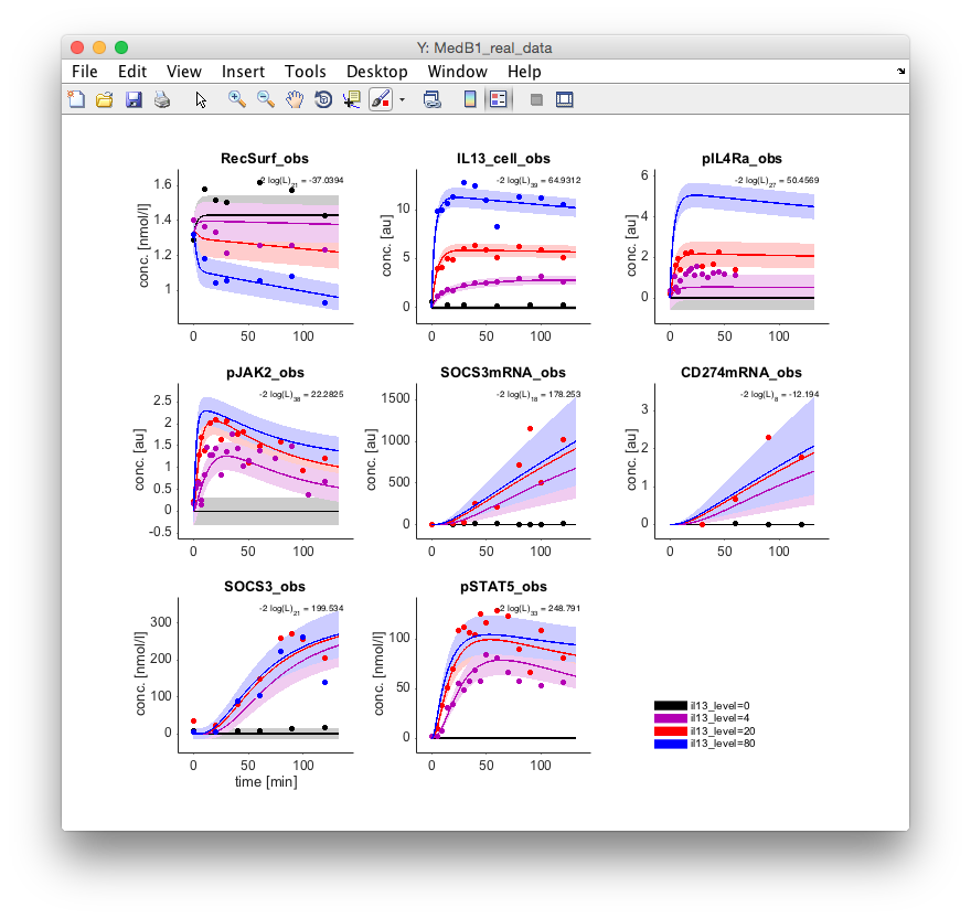
One way to also visualize the underlying ODE solutions is to invoke arPlotter, which
opens a small graphical user interface that allows selecting data sets and available
quantities to display by the arPlot command.

The list contains the data set name (dataset), its current log-likelihood value (-2*log(L)),
the number of data points in this data set, the number of experimental conditions, if the
data plot is shown (PlotY), if the internal model dynamics are shown (PlotX), if the model
reaction fluxes are shown (PlotV), if the data set if plotted on a log10 y-axis (PlotLog), if it
is fitted on a log10 y-scale (FitLog) and if it is fitted at all (Fit).
After activating the checkbox PlotX and hitting the button Update Plots a new figure is
opened showing the dynamics of the internal variables.
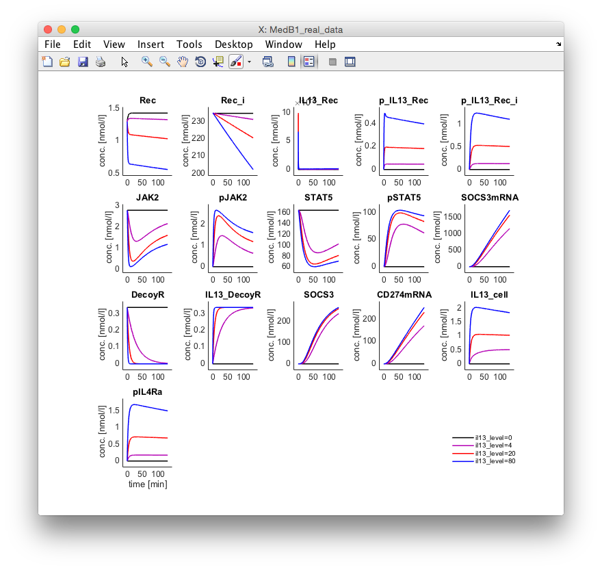
All commands executed in the Data2Dynamics framework via a graphical user interface can of course also be performed at the MATLAB command line, which enables the creation of analysis workflows.
arFit starts the selected numerical optimization algorithm to calibrate the model to the
experimental data. Several optimizers ar.config.optimizers can be selected specified by
adjusting the index ar.config.optimizer. If the option flag in the global variable
ar.config.showFitting = true model calibration is shown for each iteration by internally
calling arPlot. In this example, optimal parameters values are already loaded from a
workspace in the setup file, see line arLoadPars. If this line is commented the parameter
values are set to default values of 0.1 as can be verified by the arPrint command. arFit
then nicely demonstrates the efficiency of the implemented optimization technique by
showing the iterative improvements.
To check whether the current local optimum is also globally optimal a sequence of n fits
for random initial guesses is executed using the command arFitLHS(n). For deterministic
optimization the initial parameter guesses are generated by random sampling. arFitLHS
replace previous values if a better fit is found. The resulting likelihoods of the n fits are
displayed in a sorted manner by arPlotFits.
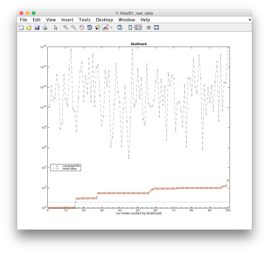
This figure shows the result for n=100 independent fits from random initial starting points
and indicates 1) the improvement of the initial likelihood value by several orders of
magnitude (gray crosses vs. red circles), and 2) the plateaus after optimization
demonstrating that local minima are reliably detected. The more often the same local
minima are found, the better the chance that all existing local minima including the global
one were found. See [Raue et al., PLOS ONE 2013](http://www.plosone.org/article/info%3Adoi
%2F10.1371%2Fjournal.pone.0074335) for further
explanation.
A convenient way to assess whether a parameter of a non-linear model has a finite
confidence region (i.e. is identifiable, see Raue et al., Bioinformatics 2009 for further explanation) is by
calculating the profile likelihood. This
concept generalizes the concept of standard errors and Fisher-Information for the
non-linear setting. After initializing the profile likelihood calculation by arPLEInit, the profiles for
all parameters are calculated automatically by ple. The calculation for a specific
parameter, e.g. for the internalization rate Rec_intern might be performed by
ple('Rec_intern', m). The second argument m can be used to specify the maximum
number of steps (default: 50) along the profile. For this example, 200 points in lower an
upper direction were calculated via ple('Rec_intern', 200).
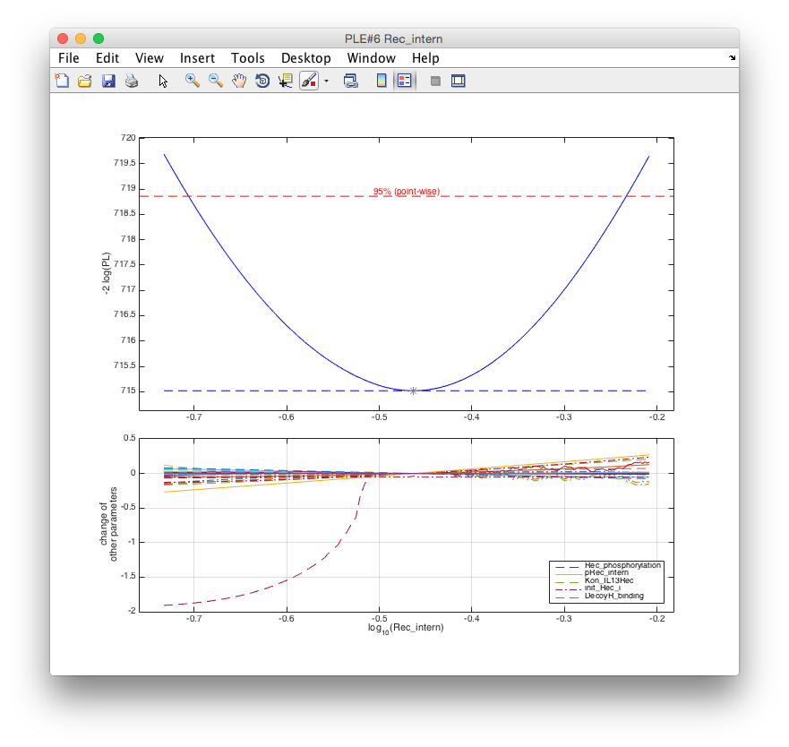
In the upper panel the profile likelihood is plotted. The parameter is identifiable because
the profile (blue line) crosses the statistical threshold (red) at both sides of the optimum.
The lower panel shows along the profile, i.e. for specific values of Rec_intern, how all
other parameters have to be adjusted to describe the data. These dependencies are of
particular interest for non-identifiabilities as demonstrated in the following example.
The second parameter examined for identifiability is the initial concentration of the IL13
receptor init_Rec_i. Here, the default settings only calculate a part of the profile of
interest. The following commands quickly provide the whole profile likelihood.
k = arPrint('init_Rec_i');			% Find index of parameter init_Rec_i
global ar; 		% Get access to global variables
ar.ub(k) = 5;						% Set upper boundary of init_Rec_i to 10^5 for MLE
ple('init_Rec_i',[],[],.1,.1)		% Calculate profile with fixed stepsize of 0.1
The resulting figure shows the profile likelihood of init_Rec_i.
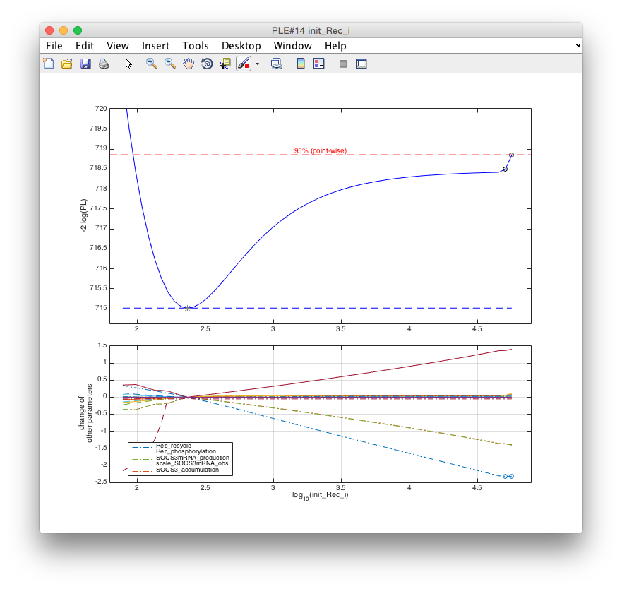
The following conclusions can be drawn from this plot:
- The parameter is significantly larger than 2 (on the log10-scale)
- The profile becomes flat for values > 4
- The increase at around 4.7 induced is due to another parameter (
Rec_recycle) hitting its lower boundary as indicated by the circles in the lower panel. To check this hypothesis, the profile is recalculated with a less stringent lower boundary for the receptor recycling parameter.
j = arPrint('Rec_recycle');		% Find index of Rec_recycle
ar.lb(j) = -8;					% Set lower boundary of Rec_recycle to 10^-8 for MLE
ple(k,[],[],.1,.1)				% Re-calculate profile of init_Rec_i
The resulting profile likelihood is flat in upper direction, which demonstrates that the
receptor concentration init_Rec_i can not be significantly restricted by the data towards
large numbers. Hence init_Rec_i is practically non-identifiable.
- Installation and system requirements
- Setting up models
- First steps
- Advanced events and pre-equilibration
- Computation of integration-based prediction bands
- How is the architecture of the code and the most important commands?
- What are the most important fields of the global variable ar?
- What are the most important functions?
- Optimization algorithms available in the d2d-framework
- Objective function, likelhood and chi-square in the d2d framework
- How to set up priors?
- How to set up steady state constraints?
- How do I restart the solver upon a step input?
- How to deal with integrator tolerances?
- How to implement a bolus injection?
- How to implement washing and an injection?
- How to implement a moment ODE model?
- How to run PLE calculations on a Cluster?